Digital Factory Simulator (DFS)
Installation
Current version: v1.1.1
Download the Digital Factory Simulator for your operating system from the MaestroHub Portal and run:
Download and install v1.1.1 the same way you installed v1.1.0 — replace the binary, or re-load the new images for the MaestroHub + DFS Stack bundle. Existing data is preserved.
What's new in v1.1.1
- Energy Monitoring Dashboard — new pre-built dashboard with OP20 station enhancements for tracking per-station and total energy consumption. See Energy Monitoring.
- OPC UA high-volume tags — 10,000 counter tags registered for high-throughput OPC UA performance tests
- MQTT high-rate counter — faster publish rate on the embedded MQTT broker
- Improved Docker hostname handling — DFS now picks up
MHUB_EXPORT_HOST, so.mhub.jsonexports use the correct connection host when DFS runs in a Docker container
- Windows
- macOS
- Linux
- MaestroHub + DFS Stack
- Download the ZIP file and extract it to a folder of your choice
- Double-click
factory-launcher.exe(or runstart-launcher.batfor console output)
The application will appear in the system tray and a browser window will open automatically to http://localhost:13005.
Right-click the system tray icon to open the dashboard, access documentation, view logs, or shut down the simulator.
All application data is stored in %USERPROFILE%\.factory-simulator\ (logs, data, and config subdirectories).
tar -xzf factory-launcher_*_darwin_arm64.tar.gz
cd factory-launcher_*_darwin_arm64
./factory-launcher
On first run, macOS may block the application. Go to System Settings > Privacy & Security and click Open Anyway. If blocked by Gatekeeper, right-click the binary, select Open, then click Open in the dialog.
The application will appear in the menu bar and a browser window will open automatically to http://localhost:13005. Click the menu bar icon to open the dashboard, access documentation, view logs, or shut down the simulator.
All application data is stored in ~/.factory-simulator/ (logs, data, and config subdirectories).
tar -xzf factory-launcher_*_linux_amd64.tar.gz
cd factory-launcher_*_linux_amd64
chmod +x factory-launcher
./factory-launcher
A browser window will open automatically to http://localhost:13005. In desktop environments with D-Bus support, a system tray icon will appear. In headless or server environments, the application runs without a tray icon. Use Ctrl+C to shut down gracefully.
All application data is stored in ~/.factory-simulator/ (logs, data, and config subdirectories).
The stack bundle is a single tarball containing pre-loaded MaestroHub Lite and Digital Factory Simulator images plus a wired-up docker-compose.yml. No internet access is required after download.
# pick the architecture matching your host (amd64 or arm64)
tar -xzf maestrohub-dfs-stack_*_amd64.tar.gz
cd stack

docker load -i maestrohub-lite.tar.gz
docker load -i digital-factory-simulator.tar.gz
docker compose up -d
Once up, the stack exposes:
| Service | URL |
|---|---|
| MaestroHub UI | http://localhost:8080 |
| DFS Dashboard | http://localhost:13005 |
| DFS MES REST API | http://localhost:18080/api/v1/ |
| DFS ERP REST API | http://localhost:18081/api/v1/ |
Industrial-protocol ports (MQTT 11883, OPC UA 14840 / 14841, Modbus 15020 / 15021, embedded PostgreSQL 15432) are bound inside the maestrohub-stack Docker network only — they are not published to the host. Other containers on the same network reach DFS via the digital-factory hostname (e.g. opc.tcp://digital-factory:14840).
To stop the stack: docker compose down (keeps data volumes) or docker compose down -v (also wipes maestrohub-data and digital-factory-data).
DFS runs directly on the host, not inside Docker. If MaestroHub is running as a Docker container, it cannot reach DFS via localhost. Use host.docker.internal instead of localhost when configuring DFS connection addresses in MaestroHub (e.g., opc.tcp://host.docker.internal:14840).
Overview
The Digital Factory Simulator (DFS) is a software application written in Go that simulates a realistic brake caliper body manufacturing line. It runs as a single binary and exposes industrial protocols (OPC UA, Modbus TCP, MQTT), REST APIs, a web dashboard, and an embedded PostgreSQL database, allowing external systems to interact with the simulated factory as if it were a real production environment.
Product
The simulated factory manufactures Front Brake Caliper Housing - Left (product code BC-2024-A), an aluminum automotive component made from Aluminum A356-T6 with a weight of 2.4 kg. The product is manufactured for an OEM Tier 1 customer.
Production Line and Architecture
The production line (ID: LINE-BC-01) consists of four stations arranged in series. Raw aluminum castings enter the line, pass through each station sequentially, and exit as finished brake caliper housings.
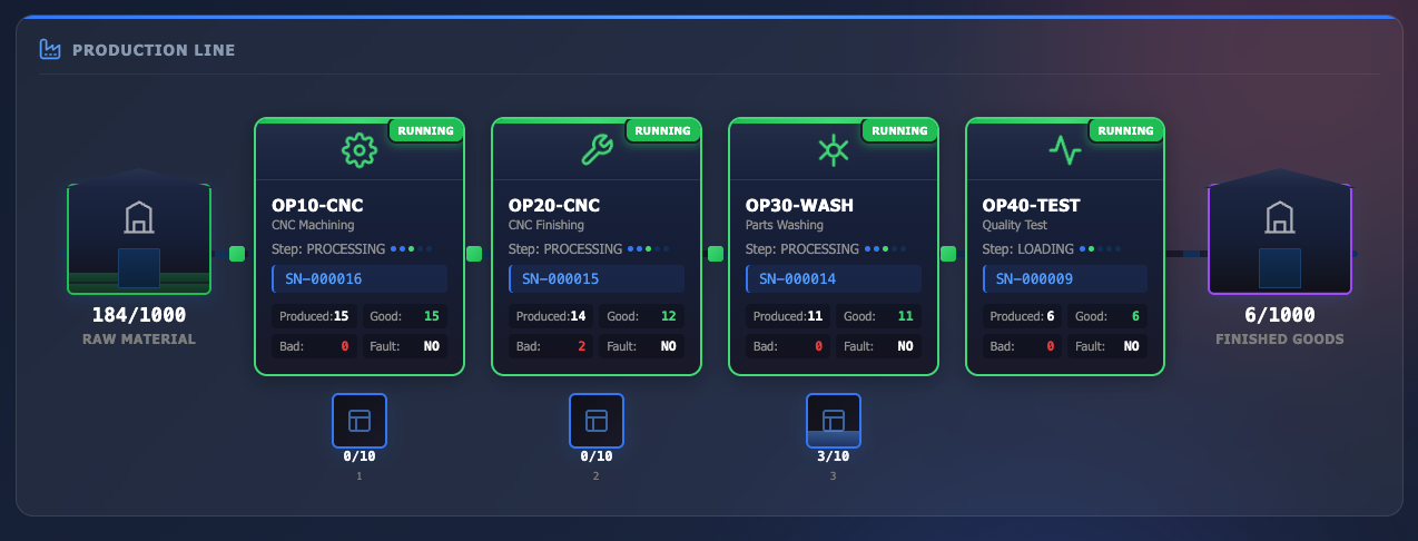
Digital Factory Simulator - Production Line
| Station | ID | Type | Protocol |
|---|---|---|---|
| CNC Rough Machining | OP10-CNC | Machining | Modbus TCP |
| CNC Finish Machining | OP20-CNC | Machining | OPC UA |
| Parts Washer | OP30-WASH | Wash | Modbus TCP |
| Leak Test | OP40-TEST | Test | OPC UA |
- OP10 (Rough Machining): Performs initial CNC machining on the raw casting using a face mill and rough bore bar.
- OP20 (Finish Machining): Performs precision CNC machining using a finish bore bar and tap, bringing the part to final dimensional tolerances.
- OP30 (Parts Washer): Cleans machining residue from the part using an industrial wash cycle with temperature, pressure, and detergent concentration control.
- OP40 (Leak Test): Performs a pressure-based seal integrity test. Parts that pass are classified as finished goods.
Buffers between stations have a capacity of 10 parts each. The raw material buffer (before OP10) and finished goods buffer (after OP40) each hold up to 1000 parts. Each part entering the line is automatically assigned a serial number (e.g., SN-000001) and is tracked through all stations for full traceability.
Stations can be in one of the following states during operation:
| State | Description |
|---|---|
| IDLE | Ready and waiting for a part |
| RUNNING | Actively processing a part (loading, machining/washing/testing, unloading) |
| FAULTED | Stopped due to a fault, resumes automatically after repair time |
| BLOCKED | Processing complete but the downstream buffer is full |
| STARVED | Ready to process but the upstream buffer is empty |
| CHANGEOVER | Tool change in progress (tool life limit reached) |
Work Orders and Operation Modes
Production is driven by work orders. Each work order specifies a target quantity of good parts to produce. Only one work order can be active at a time. When the number of good parts reaches the target, the work order is automatically completed.
DFS provides two operation modes that control how logistics and work order management are handled:
Manual mode (default) requires the operator to perform all logistics operations through the web dashboard or REST APIs:
- Loading raw materials into the raw material buffer
- Shipping finished goods from the finished goods buffer
- Creating and starting work orders
Automatic mode enables a rule-based automation engine that handles these operations based on configurable thresholds:
| Rule | Default Behavior |
|---|---|
| Raw material replenishment | When the raw material buffer drops below 100 parts, 100 parts are automatically added |
| Finished goods shipment | When the finished goods buffer exceeds 50 parts, 25 parts are automatically shipped |
| Work order start | When the current work order completes, the next planned work order starts automatically |
| Work order creation | When fewer than 3 planned work orders remain, a new work order for 10 parts is created |
The operation mode only affects logistics and work order management. Station behavior (machining, fault handling, quality checks) remains the same in both modes. The mode can be switched at any time without restarting the simulation.
Simulation Profiles
Simulation profiles control the overall behavior of the factory, including fault frequency, repair time, cycle speed, defect rates, and energy efficiency. DFS includes seven predefined profiles. The active profile can be changed at runtime through the web dashboard or REST APIs, and the change takes effect immediately without restarting.
| Profile | Expected OEE | Description |
|---|---|---|
| world_class | 85%+ | Minimal downtime (MTBF 20 min, MTTR 1 min), high efficiency (98%), and low defect rate (0.5%). Represents a well-optimized lean manufacturing environment. |
| typical | 65-75% | Moderate fault frequency (MTBF 10 min, MTTR 3 min), 90% cycle efficiency, and 2% defect rate. Represents an average real-world factory with room for improvement. |
| struggling | 45-55% | Frequent faults (MTBF 5 min), slow cycles (75% efficiency), and high defect rate (5%). Suitable for testing monitoring and alarm systems. |
| demo | Variable | Ultra-fast mode with 5x cycle speed, 1 min MTBF, and 6 sec MTTR. Produces data rapidly, making it ideal for demonstrations and quick testing. |
| availability_problem | Low availability | Very frequent faults (MTBF 3 min) with long repair times (MTTR 5 min), but good quality (1% defect rate) when running. Focus area: maintenance improvement. |
| quality_problem | Low quality | High uptime (MTBF 15 min) but 12% defect rate. Focus area: quality control and SPC systems. |
| performance_problem | Low performance | Reliable machines but 65% cycle efficiency (35% slower than ideal). Focus area: cycle time optimization. |
Each profile affects OEE through a different component. The availability_problem, quality_problem, and performance_problem profiles are designed to isolate specific OEE loss categories for targeted analysis.
Exposed Interfaces
DFS exposes data through multiple industrial and IT protocols. The application follows a single-source-of-truth design where a central state object holds all production data. The simulation engine writes to this state while protocol servers read from it. State changes are propagated to subscribers through an event-driven mechanism.
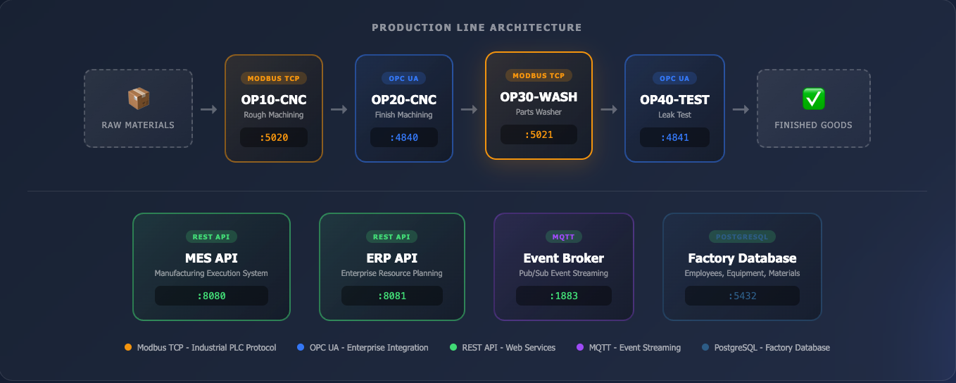
Digital Factory Simulator - Exposed Interfaces
All ports are configurable through the YAML configuration file or CLI parameters. The values shown in DFS documentation and web dashboard reflect defaults and may differ in your deployment.
OPC UA
Two OPC UA servers are available, one for OP20 (CNC Finish Machining) and one for OP40 (Leak Test). Data points include station state, process step, part counters, sensor values (spindle speed, load, feed rate, coolant, vibration, temperature), test parameters (pressure, leak rate), energy readings, fault status, time tracking, and tool information. All OPC UA nodes are read-only.
Modbus TCP
Two Modbus TCP servers are available, one for OP10 (CNC Rough Machining) and one for OP30 (Parts Washer). Register data covers station state, part counters, sensor readings (scaled integers), energy values, tool life, line counters, time tracking, and work order progress.
MQTT
An embedded MQTT broker provides event-driven and periodic topics. Event-driven topics fire on state changes, cycle start/complete, faults, part completion, work order events, and quality defects. Periodic topics publish production status, equipment status, buffer levels, and work order status every 5 seconds.
REST APIs
Two REST APIs are available:
MES API: Provides endpoints for master data (factory, products, equipment, downtime reasons, defect codes), production management (work orders, production records, counters), quality records, downtime events, real-time equipment and buffer status, energy readings, and simulation profile control.
ERP API: Provides endpoints for inventory management (raw materials, WIP, finished goods, receiving, shipping), stock movements, automation control (mode switching, rule configuration), and simulation profile management.
PostgreSQL
An embedded PostgreSQL instance contains static reference tables: departments, employees, shifts, skills, equipment, maintenance schedules/records, suppliers, materials, customers, products, BOM items, and quality specifications. PostgreSQL data is not synchronized with live simulation data and provides reference data only.
Import and Export
The DFS web application includes an API Docs page with a MaestroHub Quick Setup section. From there, you can download a pre-configured .mhub.json file that contains everything needed to start working with DFS data in MaestroHub:
| Resource | Count | Description |
|---|---|---|
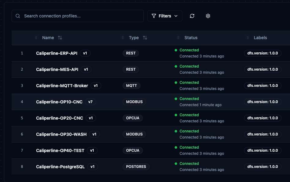
| Connections | 8 | OPC UA (OP20, OP40), Modbus TCP (OP10, OP30), MQTT Broker, MES REST API, ERP REST API, PostgreSQL |
| Functions | 136+ | All data acquisition functions across all connections (Modbus registers, OPC UA nodes, REST endpoints, SQL queries) |
| Pipelines | 4 | Station Collector (5s), Operations Collector (30s), Reference Data Collector (5min), ERP Collector (30s) |
| Dashboards | 1 | DFS OEE Monitoring — real-time OEE monitoring with 11 panels |
This file can then be imported into MaestroHub through the UI, which automatically creates all resources with no manual setup needed.
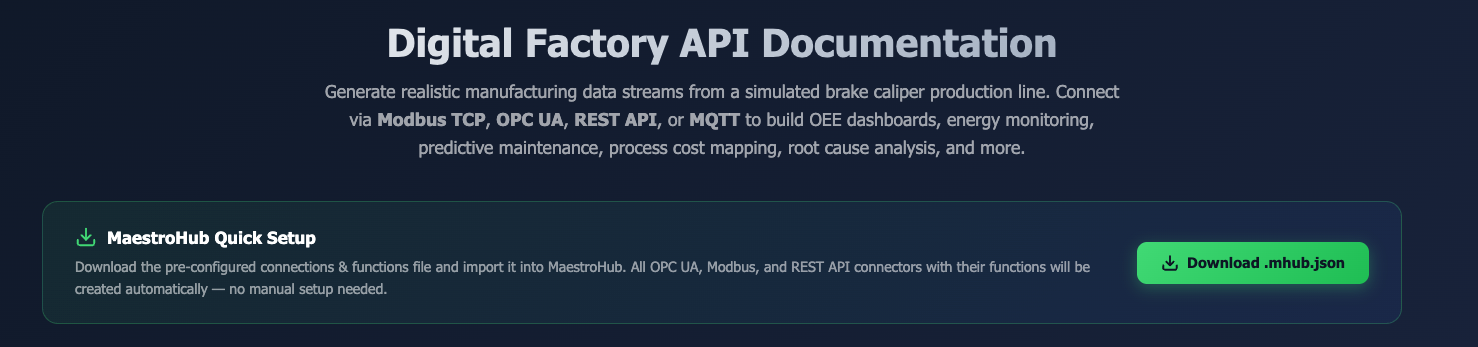
MaestroHub Quick Setup on the DFS API Docs page
To import the downloaded file into MaestroHub, navigate to System Management > Export/Import and use the Import Configuration section. Click Start Import, select the .mhub.json file, and MaestroHub will validate and resolve any conflicts automatically.
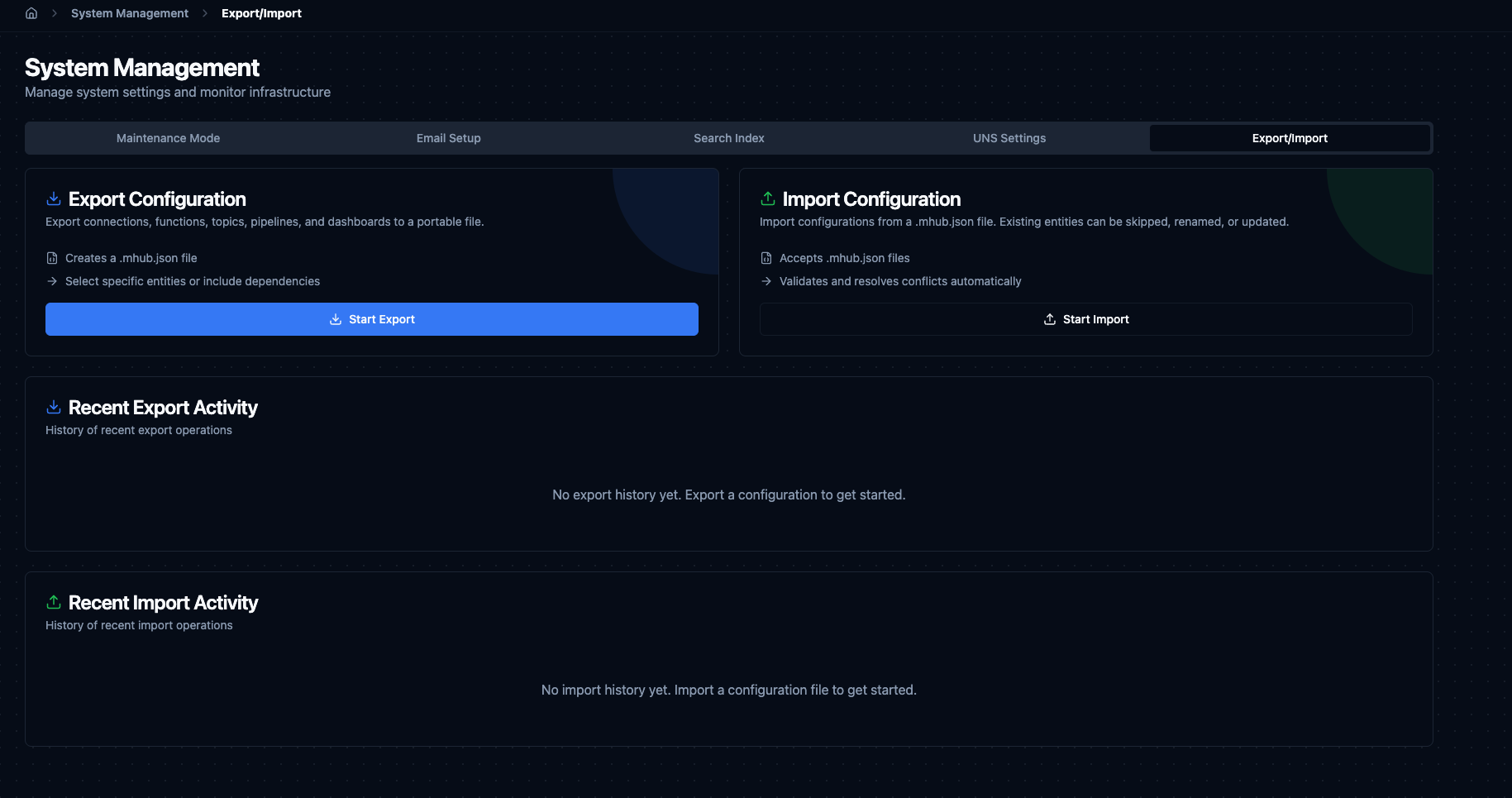
MaestroHub Import Configuration page
Once the import is complete, all DFS connections, pipelines, and dashboards are listed in MaestroHub, ready to use. The four data pipelines begin collecting data automatically and the OEE dashboard is immediately available.
DFS connections after import in MaestroHub
What the Pipelines Do
The imported pipelines transport all DFS data into the MaestroHub Unified Namespace (UNS) in a use-case agnostic structure. Each pipeline has a single responsibility and polls at a frequency matching the data's rate of change:
| Pipeline | Frequency | Source | Data |
|---|---|---|---|
| Station Collector | 5s | Modbus + OPC UA | All real-time machine tags: status, counters, faults, energy, CNC parameters, tool wear, axis positions, process values (136 tags/cycle) |
| Operations Collector | 30s | MES REST API | Active work order, buffer levels, quality records, downtime events/faults, active staff |
| Reference Data Collector | 5min | MES + PostgreSQL | Equipment master data (ideal cycle times), products, materials, BOM, maintenance schedules, shifts, departments, skills |
| ERP Collector | 30s | ERP REST API | Inventory levels (raw, finished), stock movements, automation status |
No duplication: real-time machine data comes from connectors only, operational data from MES only, reference data from PostgreSQL only, inventory from ERP only.
What the Dashboard Shows
The imported DFS OEE Monitoring dashboard provides real-time OEE monitoring with a station selector variable. All panels calculate from UNS data within the selected time range:
- LINE OEE — A × P × Q for the full line (bottleneck-based)
- Station OEE / Availability / Performance / Quality — per-station gauges
- Production Counters — parts produced, good, reject in the selected window
- State Timeline — color-coded state transitions
- Fault Status / History — current and historical fault events
- Downtime Breakdown — pie chart of time spent in each state
- Production Progress — active work order with progress bar
For a detailed explanation of each panel, how OEE is calculated, and how to interpret the data, see the DFS OEE Monitoring Dashboard guide.
Use Cases
The following use cases can be implemented using DFS as the data source and MaestroHub as the integration and orchestration platform.
OEE Monitoring
OEE (Overall Equipment Effectiveness) measures manufacturing productivity through three components:
- Availability: Derived from station run time, down time, and idle time values exposed through OPC UA, Modbus, and MQTT.
- Performance: Calculated by comparing actual parts produced against ideal cycle time targets.
- Quality: Ratio of good parts to total parts produced, using the quality outcome data from each station.
DFS simulation profiles are designed to produce different OEE characteristics. Switching between profiles such as world_class (85%+ OEE), typical (65-75% OEE), and struggling (45-55% OEE) allows you to observe how each OEE component responds to different factory conditions. The availability_problem, quality_problem, and performance_problem profiles isolate individual OEE loss categories for targeted analysis.
The imported .mhub.json includes a ready-to-use OEE dashboard. See the DFS OEE Monitoring Dashboard guide for details on how each metric is calculated and how to read the panels.
Energy Monitoring
DFS generates per-station energy consumption data including instantaneous power (kW), cumulative energy (kWh), voltage, current, and power factor. These values change based on the station's operational state (idle, loading, processing, unloading, faulted) and are available through all exposed protocols.
Using MaestroHub, you can collect energy readings from each station, calculate total line consumption, track energy cost based on peak/off-peak rates, and build dashboards that correlate energy usage with production output such as kWh per part.
Predictive Maintenance
DFS simulates tool wear progression and its effects on sensor readings. As tools approach their life limits, vibration and spindle load values increase, and defect rates rise. Faults are generated based on MTBF with an exponential distribution, meaning fault probability increases over time since the last failure.
Using MaestroHub, you can collect tool life counters, vibration trends, and spindle load data over time to build predictive maintenance workflows. By monitoring these signals, you can detect patterns that precede tool failures or quality degradation and trigger alerts before unplanned downtime occurs.
Root Cause Analysis
Every defective part produced by DFS includes a root cause classification. Each station type has its own root cause distribution. For example, machining stations attribute defects to causes such as tool wear, vibration, thermal drift, process drift, material defects, setup errors, and operator errors, each with a defined probability.
Using MaestroHub, you can aggregate defect events from MQTT or REST APIs, correlate them with station sensor data and tool life status at the time of the defect, and build Pareto charts or dashboards that highlight the most frequent root causes per station.